CO₂ and Temperature: What is the Correlation?

(c) 2009 by Barton Paul Levenson

Some global warming deniers claim that the correlation between temperature and carbon dioxide is vague and coincidental. I'll check that here with what's called a "linear regression." This means essentially that I take two columns of numbers and graph them against each other (in mathematical space if not actually on a screen or paper), and then find the straight line that comes closest to all the points. I can then compute how "significant" the regression is, which means how likely the relationship was to come about by chance. In general statisticians look for a probability of 5% or less that the relationship is due to chance, or "p < 0.05". If you achieve that, chances are you have something real going on.

The raw data is in a table below. The columns are:

• Year.
• Anom is the mean global annual "temperature anomaly" measured by the NASA GISTEMP project ("NASA GISS" figures, GISS being the Goddard Institute for Space Sciences). The value are in hundredths of an absolute degree (centikelvins). The temperature anomaly is defined as the difference between the temperature for that year and the mean in some base period (this data uses the mean for 1961-1990 as the base figure).
• ln CO₂ is the natural logarithm of the CO₂ level. Radiation physics says the radiative forcing from accumulated carbon dioxide should be related to the log of the level rather than the level itself, so this is what we actually use in the computation.
• CO₂ is the actual carbon dioxide level, since ln CO₂ is a little hard to visualize. The values are in parts per million of the atmosphere by volume. The source is Law Dome ice core readings for 1880 to 1958 and Mauna Loa CO₂ observatory readings for 1959-2007. The figure for 1964 was interpolated by yours truly.

Here's the actual data:

Year	Anom	lnCO2	CO2
1880	-12	5.6723	290.7
1881	-12	5.6740	291.2
1882	-1	5.6757	291.7
1883	-5	5.6771	292.1
1884	-43	5.6788	292.6
1885	-24	5.6802	293.0
1886	-26	5.6812	293.3
1887	-46	5.6822	293.6
1888	-24	5.6829	293.8
1889	6	5.6836	294.0
1890	-21	5.6843	294.2
1891	-55	5.6846	294.3
1892	-39	5.6853	294.5
1893	-40	5.6856	294.6
1894	-33	5.6860	294.7
1895	-33	5.6863	294.8
1896	-27	5.6866	294.9
1897	-16	5.6870	295.0
1898	-20	5.6877	295.2
1899	-25	5.6887	295.5
1900	-6	5.6897	295.8
1901	-5	5.6907	296.1
1902	-30	5.6920	296.5
1903	-36	5.6931	296.8
1904	-42	5.6944	297.2
1905	-26	5.6958	297.6
1906	-15	5.6974	298.1
1907	-40	5.6988	298.5
1908	-30	5.7001	298.9
1909	-31	5.7014	299.3
1910	-21	5.7028	299.7
1911	-25	5.7041	300.1
1912	-33	5.7051	300.4
1913	-29	5.7064	300.8
1914	-3	5.7074	301.1
1915	5	5.7084	301.4
1916	-20	5.7094	301.7
1917	-47	5.7108	302.1
1918	-35	5.7118	302.4
1919	-9	5.7127	302.7
1920	-17	5.7137	303.0
1921	-5	5.7151	303.4
1922	-10	5.7164	303.8
1923	-17	5.7174	304.1
1924	-12	5.7187	304.5
1925	-16	5.7203	305.0
1926	4	5.7216	305.4
1927	-6	5.7229	305.8
1928	-1	5.7246	306.3
1929	-23	5.7262	306.8
1930	-4	5.7275	307.2
1931	2	5.7291	307.7
1932	4	5.7307	308.2
1933	-11	5.7320	308.6
1934	5	5.7333	309.0
1935	-8	5.7346	309.4
1936	2	5.7359	309.8
1937	12	5.7366	310.0
1938	15	5.7372	310.2
1939	-2	5.7375	310.3
1940	14	5.7379	310.4
1941	11	5.7379	310.4
1942	10	5.7375	310.3
1943	6	5.7372	310.2
1944	10	5.7369	310.1
1945	-1	5.7369	310.1
1946	0	5.7369	310.1
1947	12	5.7372	310.2
1948	-3	5.7375	310.3
1949	-9	5.7382	310.5
1950	-17	5.7388	310.7
1951	-2	5.7401	311.1
1952	4	5.7414	311.5
1953	12	5.7427	311.9
1954	-9	5.7443	312.4
1955	-8	5.7462	313.0
1956	-18	5.7481	313.6
1957	8	5.7500	314.2
1958	9	5.7523	314.9
1959	5	5.7557	316.0
1960	-2	5.7586	316.9
1961	10	5.7609	317.6
1962	5	5.7635	318.5
1963	2	5.7652	319.0
1964	-25	5.7668	319.5
1965	-15	5.7684	320.0
1966	-8	5.7726	321.4
1967	-2	5.7750	322.2
1968	-9	5.7778	323.1
1969	0	5.7827	324.6
1970	4	5.7859	325.7
1971	-10	5.7879	326.3
1972	-5	5.7913	327.5
1973	18	5.7981	329.7
1974	-6	5.7998	330.3
1975	-2	5.8026	331.2
1976	-21	5.8056	332.2
1977	16	5.8108	333.9
1978	7	5.8156	335.5
1979	14	5.8196	336.9
1980	28	5.8251	338.7
1981	40	5.8287	339.9
1982	9	5.8323	341.1
1983	34	5.8371	342.8
1984	15	5.8419	344.4
1985	12	5.8462	345.9
1986	19	5.8498	347.2
1987	35	5.8549	348.9
1988	42	5.8622	351.5
1989	28	5.8662	352.9
1990	48	5.8698	354.2
1991	44	5.8738	355.6
1992	15	5.8760	356.4
1993	19	5.8778	357.0
1994	32	5.8830	358.9
1995	46	5.8885	360.9
1996	39	5.8934	362.6
1997	41	5.8965	363.8
1998	72	5.9044	366.6
1999	46	5.9089	368.3
2000	42	5.9121	369.5
2001	57	5.9163	371.0
2002	68	5.9218	373.1
2003	67	5.9286	375.6
2004	60	5.9333	377.4
2005	76	5.9393	379.7
2006	66	5.9450	381.8
2007	74	5.9495	383.6

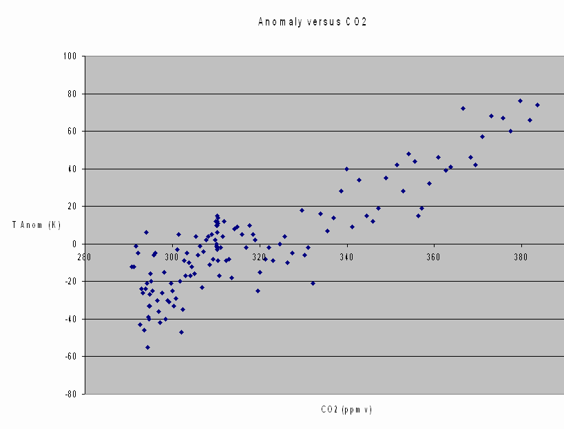
Here's the data in a graph:

The units for temperature anomaly should be cK, of course, not K. Sorry about that. Excuse the fuzziness; it's a .gif file.

I used Microsoft Excel to run the regression. The data points covered the period from 1880 to 2007 inclusive, so there were N = 128 data points. The regression line I found was:

The numbers in parentheses are "t-statistics," and they measure how significant the numbers above them are. The coefficient of the CO₂ term is significant at p < 2.4483 x 10^-41. That means the chances against the relationship being coincidental are less than 1 in about 4 x 10⁴⁰.

The correlation coefficient is about 0.874, which means 76.4% of the variance is accounted for. Every other factor that affected temperature during this time span, then, accounted for 23.6%.

More than coincidence? You be the judge!

Note added 15 March 2009:

Some half-educated global warming deniers pointed out that I didn't account for "autocorrelation in the residuals" in my regression, and said that my analysis was therefore invalid. There is something called the "spurious correlation problem" when dealing with two series increasing over time--they may seem to be correlated just because both are rising. There are ways to compensate for this. I performed a technique called "Cochrane-Orcutt iteration" in which I adjusted the regression coefficients using a factor called the "estimated autocorrelation coefficient of the residuals."

This factor, designated ρ with a circumflex over it or "rho-hat," measures the tendency of positive errors in the estimate to be followed by positive errors again, or negative errors by negative errors, and so on. Rho-hat for the regression above is about 0.4, so I transformed the two data series using an equation in rho-hat and ran the regression again, which gave a different, smaller figure for rho-hat. I repeated until the results stabilized. Rho-hat was down to insignificant levels (less than 0.1). The regression was no longer optimal by the simple least-squares criterion, but it still accounted for 60% of the variance.

So changes in carbon dioxide are still heavily linked to changes in temperature, and the correlation is not vague and coincidental. That was all I was trying to prove, and that point stands.

Thanks to David A. Benson for letting me know what was being said in the blogs.