(c) 2017 by Barton Paul Levenson
Regression finds the effect of one or more "independent variables" (X2, X3, etc.) on one "dependent variable," Y. We'll get to the missing X1 later.
Start with a sample of points, where each point has a value for Y, X2, and any other Xs. For instance, you might have several years of economic data for some country--perhaps the inflation rate for Y, money supply growth rate for X2, and real economic growth rate for X3.
By doing certain math operations on these columns of numbers, we can estimate what influence each independent variable has on the dependent variable--how much "variance" in Y the various Xs explain, or how much they all explain together, and in which directions. This lets us test theories about such relationships. Is money growth related to inflation? Rising CO2 to rising temperatures? Studying such things often starts with regression analysis.
Several things can go wrong with regression, but there are statistics designed to test for such problems.
To explain how it all works, we have to use matrix math. See Appendix 3 ("Grossly Oversimplified Matrix Math Course") if you don't know it.
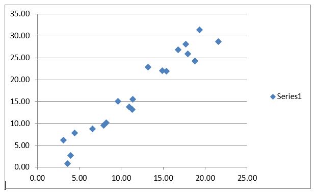
Regression produces a statistical equation relating Y to one or more Xs. It isn't an exact equation, like a natural law, that can be reversed to give the original variables perfectly. In real-world data there is "noise" as well as "signal," and it shows up in regression results. The cause of some phenomenon may be very complex and you may be missing some variables. Or some observations may be mistaken. So if you plot the data on a graph, it won't all fall on a perfectly straight line. There will be a "cloud" of points that only suggest a relationship. So how do you find the best line to represent all the points?
Regression, invented by Carl Friedrich Gauss c. 1800, finds the line that comes as close as possible to all points on the graph. It uses the "least squares criterion:" The line of best fit minimizes the sum of the squared deviations of each point. The deviations are the minimum distances from each point to the line.
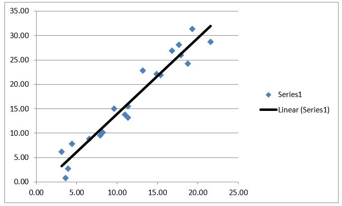
Why squared? Well, if you use the raw deviations, the positive and negative deviations above and below the line just cancel out. But if you square them, you get a positive number on each side of the line. The group's mean distance from the line can then be minimized using calculus. Gauss did the minimization and found the equations now used for regression.
We want to estimate the coefficients of this "regression equation:"
Y = β1 + β2 X2 + β3 X3 ... + βN XN + ε
Here, the βs are constant "regression coefficients" which tell you how much each X affects Y on average--there may be only one X in a simple Y-on-X regression. The ε is the error term you need to exactly fit each Y value. Without the error term, the regression equation only gives you Ŷ, the estimated value of Y for a point, given the known Xs.
You start by filling two matrices with the raw data. The Y vector takes all the Y values. The X matrix takes the X values, with the values for X2 in the second column, X3 in the third column, and so on. The first column, X1, gets filled with all 1s. You need this to calculate the equation's "intercept," or constant term, β1.
Here's how X and Y would look for a regression of Y on two variables, X2 and X3, with four observations (four points) available. Each row represents one point or observation. Each column represents a variable:
    │ 1st Y │         │ 1    1st X2    1st X3 │
Y = │ 2nd Y │     X = │ 1    2nd X2    2nd X3 │
    │ 3rd Y │         │ 1    3rd X2    3rd X3 │
    │ 4th Y │         │ 1    4th X2    4th X3 │
Using matrix math (see Appendix F), you then calculate more matrices. First you find the transpose of X, X'. Then find X' times X, which gives you the square matrix X'X. Find X'Y as well. Find the inverse of X'X, (X'X)-1.
One more matrix multiplication then gives you the vector of regression coefficients:
β = (X'X)-1 X'Y
More such equations give you the sum of squares due to regression, error, and their total:
SSR = b'X'Y - N (Ȳ)2 SST = Y'Y - N (Ȳ)2 SSE = SST - SSR
Here Ȳ is the mean value of Y for your sample. N is the number of data points.
Dividing SSR and SSE by their respective "degrees of freedom" gives you the "mean squares" MSR and MSE. The degrees of freedom are k - 1 for MSR and N - k for MSE, where k is the number of Xs in your regression, including X1. Thus:
SSR MSR = ——— k - 1 SSE MSE = ——— N - k
The coefficient of determination, R2, measures the overall "goodness of fit" for the regression:
SSR R2 = ——— SST
R2 tells you how much of the "variance" of Y your equation accounts for. Amateurs playing with regression often try to maximize R2 by adding more variables, transforming the variables different ways, etc. But high R2 doesn't always mean you've found the real relationship (if any) among the variables. You still need to test the "significance" of the regression.
One problem is that R2 never decreases by adding a new X, even if that X has no real-world effect on Y. Just by random chance, some of your newly added variable will "covary" with some of Y. But an "adjusted" R2 compensates for this effect:
N - 1 R̄2 = 1 - (1 - R2) ——— N - k
Fisher's F statistic tests the overall significance of the regression:
MSR F = ——— MSE
The degrees of freedom for F in the numerator and denominator, respectively, are:
d1 = k - 1 d2 = N - k
Most statistics textbooks include tables of significant values of F for various sample sizes. Some are on-line. For example: For a sample size of N = 30 and a regression with k = three variables (one Y and two Xs), a value of F2,27 = 3.66 or higher is significant at the 95% confidence level (p < 0.05).
The t test:
First, find the "covariance matrix" D:
D = MSE (X'X)-1
The square roots of the values along the main diagonal of D are the standard errors "se" for each regression coefficient. Student's t-statistic then tests the significance of each β:
β t = —— se
Note 06/21/2022. The phrase above in italics was inadvertently left out of the previous draft of this web page. Apologies for misleading everybody.
As with F, you can find t tables in textbooks and on-line. For example: For a sample size of N = 30, a value of |t| ≥ 2.042 is significant at the 95% level.
The Partial-F test:
This tests if adding a new explanatory variable, or several, adds significantly to your regression or not. H0 is your null hypotheses (none of the new ones help), and Ha is the alternative hypothesis (at least one does help). You need to run two regressions:
The reduced (R) model, with g independent variables: Ŷ = β0 + β1 x1 + β2 x2 ... + βg xg The full (F) model, with k independent variables: Ŷ = β0 + β1 x1 + β2 x2 ... + βg xg + βg+1 xg+1 ... + βk xk H0: βg+1 = βg+2 = ... βk = 0 Ha: at least one of above <> 0
Then calculate this statistic:
(SSER - SSEF) / (k - g) F = ————————————— SSEF / (N - [k + 1])
This has F distribution with
k - g degrees of freedom for the numerator, and N - (k + 1) degress of freedom for the denominator.
Reject H0 if F is greater than the proper critical value.
| Page created: | 04/13/2017 |
| Last modified: | 06/21/2022 |
| Author: | BPL |