(c) 2017 by Barton Paul Levenson
Given two variables, and numerical values for several points--plus a theory that one variable affects the other--you can use one variable to predict the other.
For example, here are the values of two variables about conditions in the US in 2010. This time I'm using real data. M is the murder rate per 100,000 inhabitants. U is urbanization, the percent of the population living in cities.
| State | M (per 100,000) | U (%) |
|---|---|---|
| CA | 4.9 | 95.2 |
| NJ | 4.1 | 94.7 |
| NV | 5.9 | 94.2 |
| MA | 3.2 | 92.0 |
| HI | 1.8 | 91.9 |
| MT | 2.1 | 55.9 |
| MS | 5.6 | 49.3 |
| WV | 3.0 | 48.7 |
| VT | 1.1 | 38.9 |
| ME | 1.8 | 38.7 |
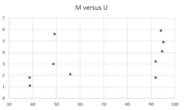
Here's how they look on a graph, with M increasing upward on the Y axis and U increasing rightward on the X axis:
The points look a little scattered.
There are two lines called regression lines we can draw on the chart:
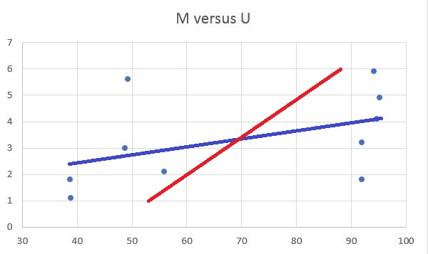
A regression line is the line that comes closest to all the points, on average. You calculate it using the "least squares criterion." This minimizes the summed squares of the deviations.
The "deviations" are the minimum distances from each point to the line. You square them because if you used linear distances, the negative values on one side of the line would cancel out the positive values on the other. Squaring the deviations solves that problem.
There are two regression lines because we're dealing with a statistical relationship between two variables, not a hard-and-fast natural law--although some natural laws have actually been discovered using regression analysis! There is both a "regression of Y on X" (the blue line in the chart, M on U) and a "regression of X on Y" (the red line, U on M).
The angle between the lines shows the correlation between the two variables. At r = 0, the lines would be at right angles to one another. For the chart above, r = 0.459, which is not a very strong correlation, so the lines are still fairly far apart. For r = 1 or -1 (perfect correlation), the lines would coincide, and there would be only one regression line. A regression line takes the following form:
4-1: Ŷ = a + b X
where Ŷ (read "Y-hat") is the estimated value of Y at a given point, X is the observed value of X, and a and b are numeric constants. You find a and b with these equations:
SSxy 4-2: b = ——— SSx2 4-3: a = x̄Y - b x̄X
Here, SSxy and SSx2 are two of the reduced sums of squares from the last chapter, defined by equations 2-2 and 2-3. x̄Y and x̄X are the mean values of Y and X, respectively.
For the other equation, the regression of X on Y, you would just alter the terms a bit:
SSxy 4-4: b = ——— SSy2 4-5: a = x̄X - b x̄Y
Regression can be extended to any number of variables. The one you want to explain is the "dependent variable." The ones you use to explain it are "independent variables." I won't go into how to calculate such a multiple regression here because it is quite complex, involving matrix math and a technique called Gauss-Jordan elimination. I give details in Appendix 4.
In this chapter I just want to discuss how to "read" a regression. I lay out the regressions in this tutorial in a table format. Here's an example:
| M = f(U) | N = 10 |
| R2 = 0.2109 | R̄2 = 0.1123 |
| F1,8 = 2.138 (p < 0.1818) | SEE = 1.605 |
| Name | β | t | p |
|---|---|---|---|
| M | 1.199 | 0.7705 | 0.4632 |
| U | 0.03075 | 1.462 | 0.1818 |
That's a lot of symbols and numbers. But if you take it slowly it's not hard to understand.
The top line gives the hypothesis: the murder rate, M, is a function of urbanization, U. There are ten points in the sample.
The next line shows R2 and R̄2. R is the "coefficient of multiple correlation," an extension of Pearson's r for several variables at once. Its square is the "coefficient of multiple determination" or just "the coefficient of determination." It says how much of the variance of our dependent variable can be attributed to the variance of the others.
The problem with R2 is, if you just add variables at random, the amount of variance accounted for will almost always go up at least a bit. R̄2 (read "R-hat squared") is "adjusted" so simply adding more variables won't always make the number go up. You often see only R̄2 for a regression in scientific articles.
The F statistic, on the next line, is a test of how "significant" the regression is. F is a "nonnegative" number; it can be anywhere from 0 up. Once you have it, you have to compare F to its critical value, based on the number of points and variables you use. Mathematical details are in Appendix 2. If your F value is below the critical value, your regression is "not significant." That means even if you seem to have a relation between your dependent and independent variables, it is probably just due to chance.
Remember the "null hypothesis" from Part 2 of the tutorial. When you test whether something is likely to be true or not, you're always testing against a null hypothesis. The null hypothesis is usually that there is no real relation--whatever you might have found is from sampling error. But if you have a statistic like F that is at or higher than the "critical value," you can "reject" the null hypothesis.
Here it is in formal notation. I'll assume two variables, Y and X, and your hypothesis is that X affects Y. If β is the regression coefficient on X, then a "two-tailed" null hypothesis is:
H0: β = 0 I think X has a real effect, so the null hypothesis is, it doesn't.
A "one-tailed" hypothesis would be that the effect is definitely higher, or lower, than 0:
H0: β ≤ 0 I think β is positive, so the null hypothesis is, it's not. H0: β ≥ 0 I think β is negative, so the null hypothesis is, it's not.
There are different critical values of the test statistic, depending on how secure you want to be. Regressions reported in science articles often put an asterisk next to a variable that is significant at the 95% level, or two asterisks for one significant at the 99% level.
How do you calculate the critical value? It's complicated. I give details in Appendix 2. But most of the time you can just look up critical values in a table. Most good statistics textbooks have tables of critical values of F, and also of the commonly used t, χ2, and DW statistics.
The F-statistic in our regression is insignificant at p < 0.18. There's one chance in five our relation is pure sampling error.
SEE is the Standard Error of Estimate, a sort of standard deviation for the regression as a whole. Our table has SEE = 1.605. Since the dependent variable, M, ranges from 1.1 to 5.9 in our sample, our estimates won't be too accurate.
In a regression, you usually want R2, R̄2and F as high as possible. You want SEE as low as possible.
Now, below the section with the overall statistics is the section with statistics on each variable:
| Name | β | t | p |
|---|---|---|---|
| M | 1.199 | 0.7705 | 0.4632 |
| U | 0.03075 | 1.462 | 0.1818 |
Name is the name of the variable. β (beta) is the regression coefficient, the multiplier for that variable in your equation (for the intercept, you just use the number). The regression equation from our table would therefore look like this:
M̂ = 1.119 + 0.03075 U
Note that M̂ means the estimated value from the regression, not the actual value.
The first line in the table gives the value of the "intercept," 1.119 in this case. 0.03075 is the coefficient of % urbanization.
This is important to know: regression equations like this are fundamentally different from equations in the natural sciences. For a physics equation like Newton's first law:
f = m a
where f is force, m mass and a acceleration, the equation applies exactly. The equals sign is a real equals; the product on the right must always exactly equal the variable on the left. Statistical equations are not like that. They hold on average only. A fully correct version of the regression equation above would be
M = 1.119 + 0.03075 U + ε
where ε is the error term--the term that has to be added so each prediction equals the actual value at that point. Note that this is an equation for M, not M̂.
The next column in the regression table gives the statistic known as Student's t, since the economist who invented it, W.S. Gossett, published his 1908 paper about it under the pseudonym "Student." The t value tests how significant each coefficient in the equation is, based, again, on sample size. Usually a t-statistic of 2 or higher (-2 or lower if negative) means your coefficient is significant at the 95% level. You can look up critical t values in the back of a statistics textbook. I show how to calculate them in Appendix 2. And I give tables of critical values--F, t, etc.--in Appendix 8.
In our example table, the intercept and the coefficient of urbanization are both statistically insignificant.
This is not a very good regression. Only a fifth of variance is accounted for, no coefficients are significant, and neither is the regression as a whole. In this form, at least, our hypothesis fails. What do you do in a case like this?
You can try increasing your sample size to overcome the small p values. If you ran this regression again with data from all fifty states, plus Puerto Rico and the District of Columbia, maybe it would support your hypothesis.
Or maybe adding other variables to the mix would improve the fit. You might make the fit quadratic (depending on U2 as well as U), or bring in income levels, or the unemployment rate, or whatever else you think might help.
But eventually, if you keep testing and your coefficient on the urbanization term never succeeds, it implies your original hypothesis was wrong. That's something all scientists have to keep in mind: Your clever idea might be wrong. That's life. Scientists who can't deal with their pet theories being wrong, who keep insisting they're right in the face of the evidence, are no longer practicing science. They have become crackpots.
| Page created: | 04/10/2017 |
| Last modified: | 04/13/2017 |
| Author: | BPL |