(c) 2017 by Barton Paul Levenson
Officially, these are "measures of central tendency and dispersion." But "simple statistics" is close enough.
We start by gathering measurements of the same type--the "sample." We wants to find summary measures that describe the whole thing. The simplest such measure is
The Count (or number).
That's just how many measurements you have. Or as statisticians say, "how many points are in your sample." The usual symbol for it is N, for number.
The Sum.
The sum, or total, of a sample is what all the individual measurements add up to. You write it like this:
Σx
The Σ (upper-case Greek letter "sigma") is not a variable, but stands for taking the sum of a series. This is called "sigma notation," and it gets used a lot in statistics. The x represents the individual data values--the "points."
Neither the number nor the sum tells you much about your sample so far. But put them together and you get something interesting: The mean or average value of the sample. The recipe for the mean is: Divide the sum by the count. Here it is as an equation:
Σx x̄ = —— N
Here the x̄ (read "x-bar") stands for the mean. So this equation reads "the mean equals the sum of the values divided by their number."
Here's an example--the percentage unemployment for the US in 2000-2004:
| Year | U (%) |
|---|---|
| 2000 | 4.0 |
| 2001 | 4.7 |
| 2002 | 5.8 |
| 2003 | 6.0 |
| 2004 | 5.5 |
If we add these figures, we get a statistic: a sum of Σx = 26.0. There are five figures, N = 5. Dividing 26.0 by 5, we get the mean unemployment rate over that period: x̄ = 26.0 / 5 = 5.2%. The mean categorizes the whole group of figures at once. We can say "the mean unemployment rate from 2000 to 2004 was 5.2 percent."
There are other measures of "central tendency," most notably the median and the mode.
The median is the figure chosen so half the observations fall above it and half below it. For our group of figures, the median would be the 5.5% in 2004, since unemployment was above that twice during the period, and below it twice.
The mode is the value that occurs most often. In this case, there was no modal figure. If our sample consisted of the numbers 3, 5, 7, 7, and 10, the mode would be 7.
People often get these measures mixed up--especially reporters and comedians. You might have heard the joke that "a survey reveals half of Americans to be of below-average intelligence." But no, without a perfectly even distribution of intelligence, that would not be true. Half of Americans (and half of any other group) are of below-median intelligence. The mean may be above or below the median, because extreme figures can pull it one way or the other. Note that for our unemployment example, the median (5.5%) is higher than the mean (5.2%).
Here's another example, the income last year of five different people:
| Person | Job Status | Income ($) |
|---|---|---|
| John | systems analyst | 65,000 |
| Bob | unemployed | 4,000 |
| Mike | does odd jobs | 10,000 |
| Akisha | data-entry clerk | 15,000 |
| Tammy | in prison most of the year | 2,000 |
The median figure here is Mike's $10,000--half the people made more than that; half made less. But the mean is $19,200, pulled way up by John's high salary. The mean here is misleading. It wouldn't really tell you much about this group to know that their average income was over $19,000. No one in it made exactly that much, and four out of five made less. Thus, while the mean is an important and useful figure, it doesn't tell us everything.
To characterize a group of figures well, we need not only measures of "central tendency," but measures of "dispersion"--some clue how the figures vary.
The standard deviation.
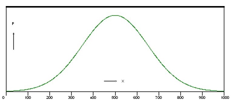
For reasons having to do with probability, an amazing number of phenomena graph out as something called a "normal distribution curve." It is also called a "Gaussian distribution" or a "bell curve," because it looks like this:
The chart shows a normal distribution curve with a mean of 500 and a "standard deviation" of 150. Here's how we define the "sample standard deviation" s:
Σx2 - (Σx)2 / N s = (————————)1/2 N - 1
The first term in the numerator under the square-root sign, Σx2, is the sum of the squares of each x value (x2 = x times x). Note the parentheses around the numerator of the next term, (Σx)2--there the sum is taken first, then that quantity is squared. Lastly, N stands for the number of values.
The standard deviation measures "dispersion;" it tells us how variable our sample is. The connection between the Bell curve and the standard deviation is this: for a "normally distributed" sample, we can predict how many figures should fall within one standard deviation of the mean, how many within two standard deviations, and so on.
Look at the bell curve. Most of the values bunch up around the mean (x̄ = 500).
Here's how many observations should fall within one or more standard deviations from the mean (rounded to three significant digits):
| s | observations (%) |
|---|---|
| 1 | 68.3 |
| 2 | 95.4 |
| 3 | 99.7 |
| 4 | ~ 100 |
In theory, the bell curve extends forever to each side of the mean, but the further you get from the mean, the less likely you are to find any values. The figure for "4 s" isn't really 100%, but just under. I rounded it off. The shape of the bell curve is such that the area under it is always equal, when expressed in the right units, to exactly 1.
It may seem crazy that a figure that extends to infinity in two directions can have a finite area under it, but trust me, the math works out that way. To explain why we'd have to get into calculus.
The greater the standard deviation, the more variable the sample is. For our unemployment figures, the standard deviation is 0.834. The standard deviation is only 16% of the mean, so this group of figures doesn't vary much. The mean is a good statistic to describe this group.
However, for the income figures in the second example, the standard deviation is $26,100. This is 137% of the mean, so that group of figures is much more variable; less uniform. The mean for this group doesn't tell us much.
The mean divided by the standard deviation is yet another statistic--the coefficient of variation, CV. CV = 0.16 for our first example and 1.37 for the second. As a rule of thumb, the mean is most useful when CV is less than 1.
| Page created: | 04/10/2017 |
| Last modified: | 04/14/2017 |
| Author: | BPL |